Cellular automata usually operate on lattices and they perform local computations, meaning the state of a cell depends on the cell’s immediate vicinity and not some global state. This means that we need some definitions of what constitutes a “vicinity” in cellular automata and agent-based models. Most of the time, the term for the direct vicinity of a cell or agent is its neighborhood.
Neighborhood relations depend on the environment that we choose for our model or automaton and our model assumptions. For instance, some specific neighborhood types are only defined for grid graphs, but not for graphs in general. The ones that we will have a look at here are called the Moore neighborhood, the Von Neumann neighborhood, and neighborhoods on graphs in general. We will approach neighborhoods only informally, but in enough detail to be useful for building agent-based models. However, I’d encourage everyone to go into more depth on your own. As you will see, this topic is closely linked with the discipline of topology. Some knowledge of topology comes in handy when building agent-based models.
Moore Neighborhood
Perhaps the most common neighborhood relation in cellular automata is the Moore neighborhood. For our checkerboard type graphs (square lattices), it looks like this:
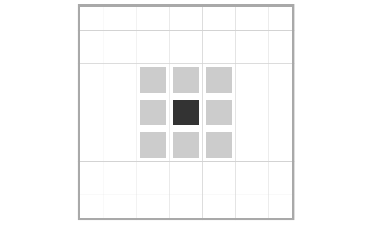
It is simply given by the four cells on each side of a cell as well as the four cells on each corner of a cell, as well as the cell itself. A convenient way to talk about the adjacent cells in the Moore neighborhood of a cell is by referring to them as cardinal and ordinal directions (north, north-east, east, south-east, south, south-west, west, north-west).
Another way you can think of the Moore neighborhood is as all squares on a chessboard that a king can reach in one move. Here you can see all the squares that the king on d5 can reach in one or two moves.
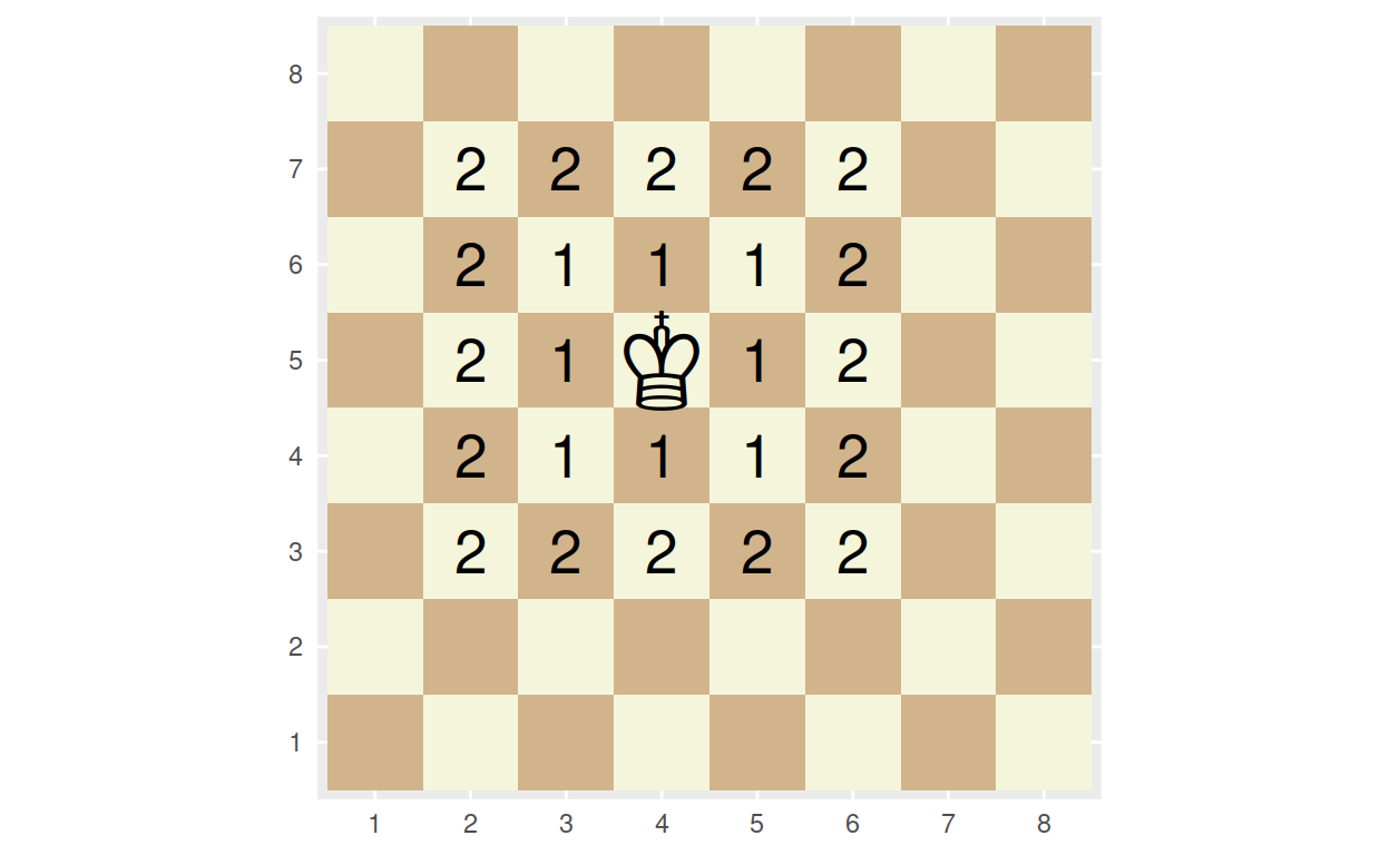
This distance metric is called the Chebyshev distance.
Once again, we have only covered some informal and basic cases of everything here. Square lattices can have higher dimensions and the Chebyshev distance is defined many way more complex vector spaces. Looking into this topic a bit more deeply and in a more formal way can be very helpful later on, but is out of the scope of this course.
Von Neumann Neighborhood
The Von Neumann neighborhood is also defined on a square lattice. On a two-dimensional lattice, it’s simply the four cells that are adjacent to each side of a cell (N, E, S, W).
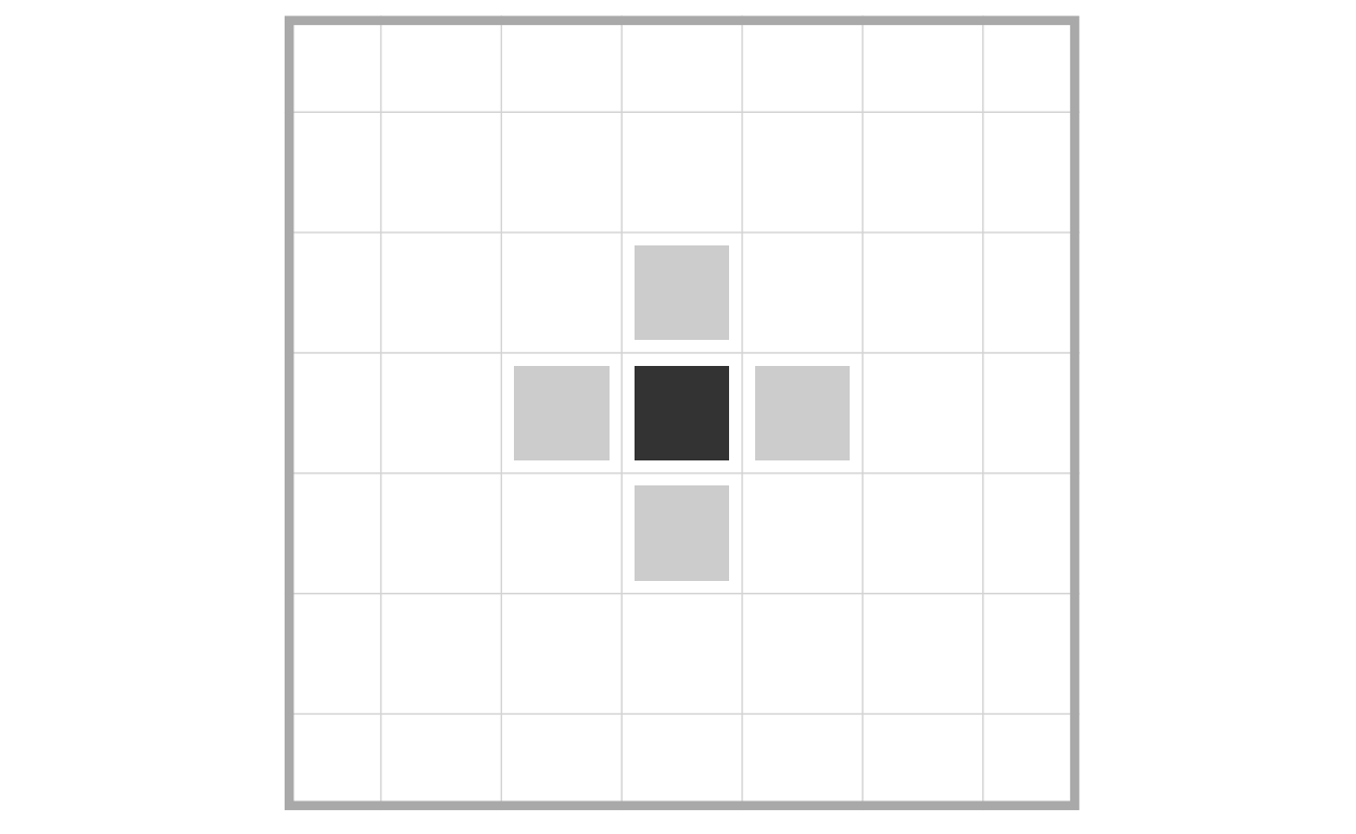
The more formal definition, however, is that the Von Neumann neighborhood of a cell is comprised all cells within a Manhattan distance of 1 as well as the cell itself. The Manhattan distance gets its name from the geometric structure of the New York district Manhattan. Blocks are organized like a checkerboard and the streets cross them accordingly. In contrast to the movement on a chessboard, however, you can’t go diagonally on a “Manhattan board” because you can’t simply go through or over the houses. Instead, you have only four directions at every intersections: N, E, S, and W.
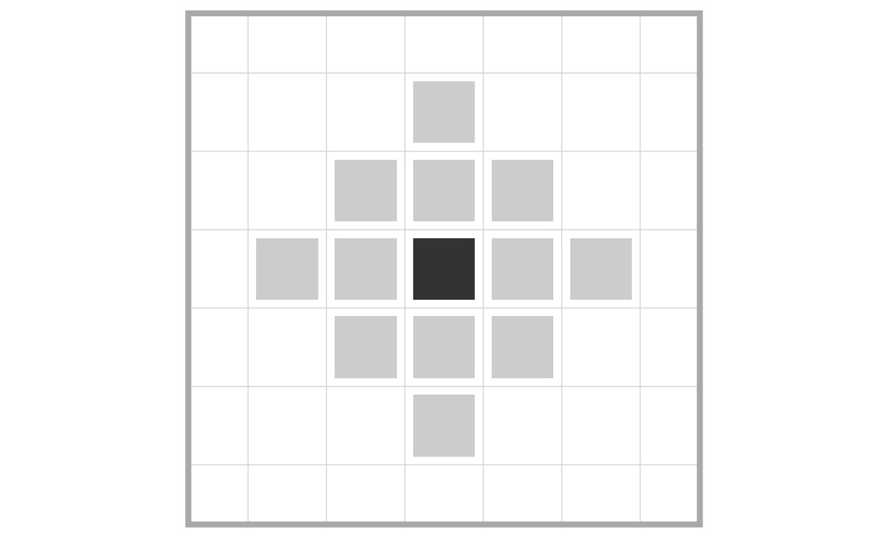
The Von Neumann neighborhood of with distance \(r = 2\) is given accordingly:
Neighborhoods in Graphs
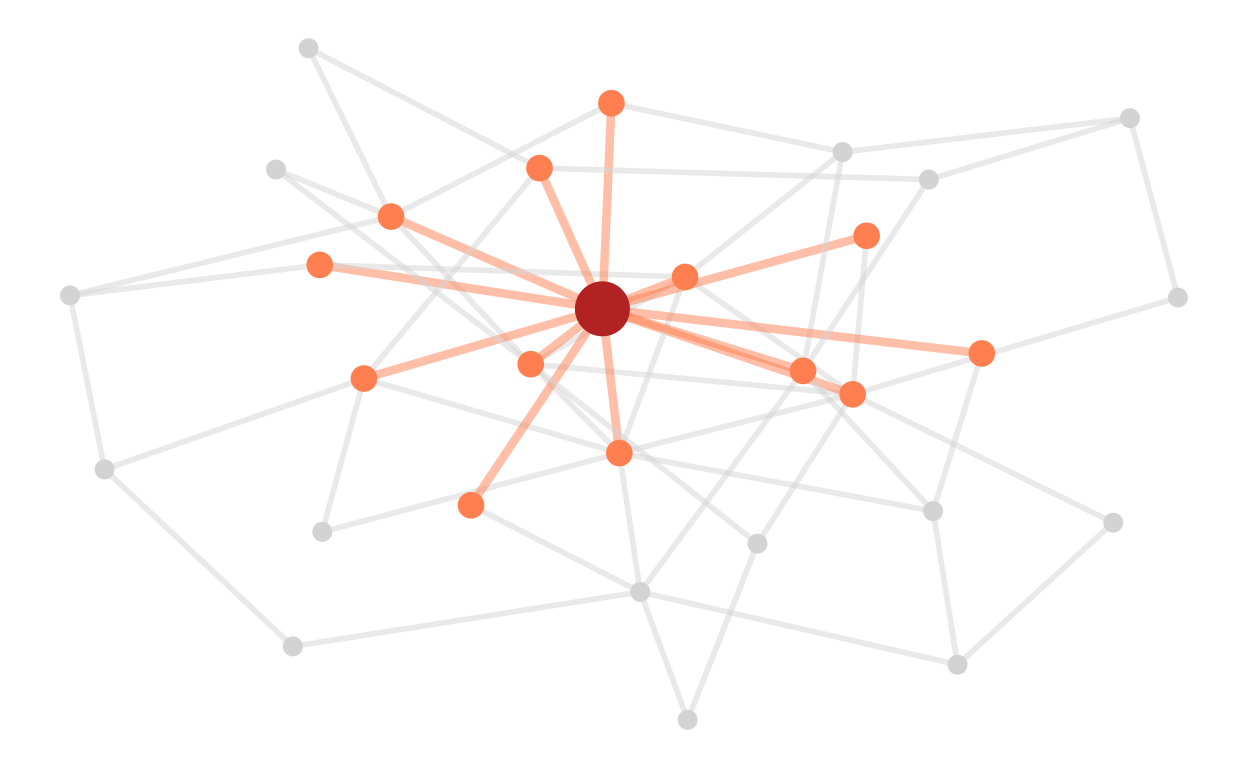
In a graph, the definition for neighborhood is pretty straight-forward. In the simplest case, it is just all nodes that are connected to a node by an edge.
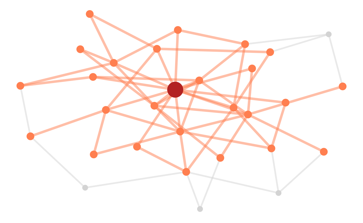
Larger distances work accordingly. The neighborhood of order 2 contains all the nodes that are at a distance of 2 from a node.
Square Lattices as Graphs