Many naturally-occurring networks have a peculiar property. Although they can be huge in terms of node count, the average path length between two nodes remains small. Really small in some cases.
If you take a social network, for instance, there are some famous experiments that show that any two nodes in the network are usually not separated by more than six degrees (the infamous six degrees of separation).
In pop science speak, this means that you are a mere six social connections away from the Queen of England.
The Erdös-Renyi model does not capture this property.
As it had been the predominant random graph model that was used for all kinds of purposes for some time, the field was ready for a new model.
The decisive innovation came from Duncan Watts and Steven Strogatz (Watts and Strogatz 1998), hence the name Watts-Strogatz model (WS model).
Start with a regular ring lattice.
This is a regular ring lattice. There are two parameters that you already have to give the WS model to construct this lattice: \(N\) is the number of nodes and \(k\) is the mean node degree.
In the case of a regular ring lattice, the mean node degree is assumed to be an even number. In colloquial terms, you construct it by arranging the nodes in a circle and attaching each node to its \(\frac{k}{2}\) neighbors on each side. That last one is a mouth full. Let’s look at it in detail.
Consider the graph above again and look at node 1. It attaches to \(2\) and \(3\) on one side and to \(10\) and \(9\) on the other. Node \(2\) attaches to \(3\) and \(4\) on the one side and to \(1\) and \(10\) on the other. You can check this for every node and see that they all attach to \(2\) other nodes on each side. Hence the parameter \(k\), in this case, is \(4\).
Here is an example with \(k = 6\):

And for good measure, here is a lattice with \(k = 2\):

Let’s return to the first graph:
Suppose the above graph is the regular ring lattice you constructed. The WS model algorithm now proceeds as follows:
First, there is yet another parameter that we need, \(\beta\). Start with node 1 now and go through each edge that attaches to it. Reroute each edge to another node with probability \(\beta\). The node to reroute to is drawn uniformly at random while avoiding self-loops. This means that you put all the other nodes (excluding the node in question, in this case node 1) in a bag and just draw a new node to attach the edge to.
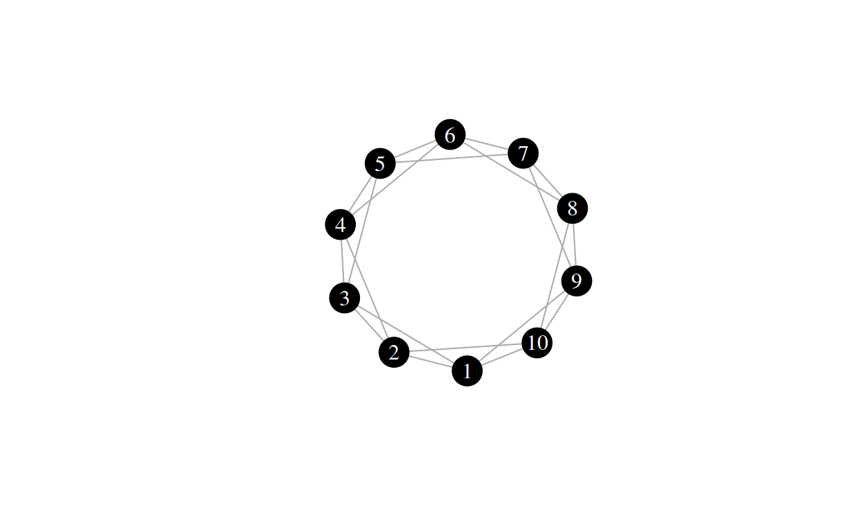
Here are some samples that were generated by this model:
\(\beta = 0.3\):

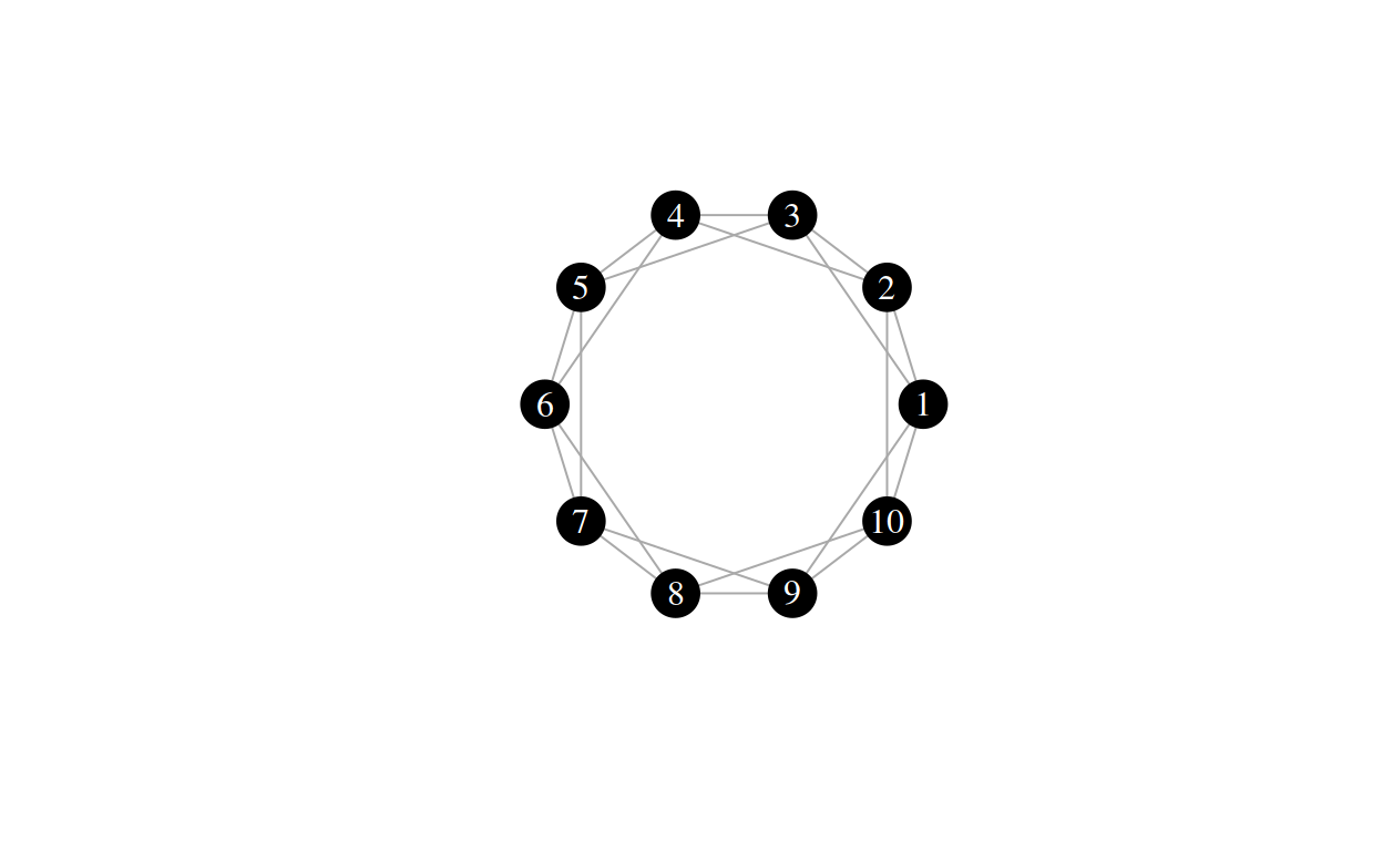
\(\beta = 0.1\)
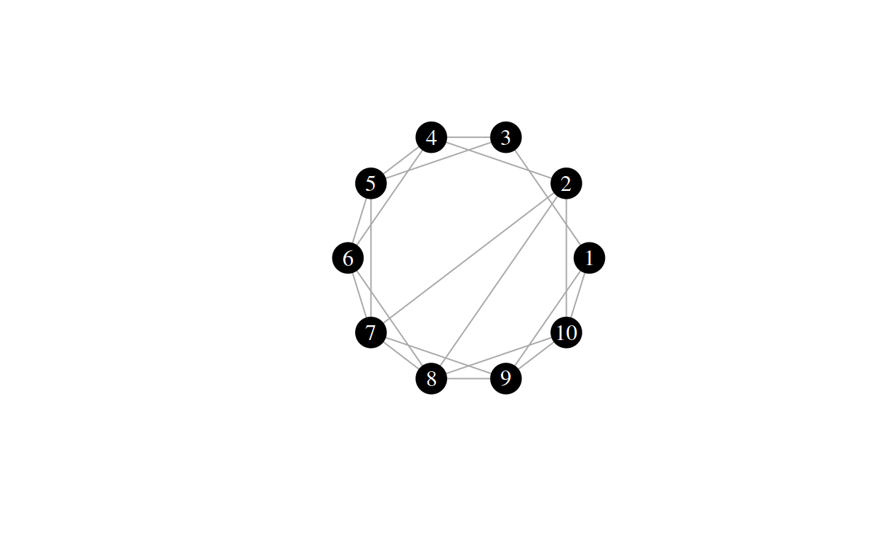
\(\beta = 0.9\)

Task
Can you guess what happens if you set \(\beta = 1\)? And what happens if you set \(\beta = 0\)? Try to figure these two questions out before you move on.
As it indicates a probability value (the re-routing probability), there are two extreme cases to the \(\beta\) parameter: \(0\) and \(1\) If \(\beta = 0\), each edge is rerouted at random with a probability of \(0\), which is - not at all. This means that the resulting graph will just be a regular ring lattice with parameter \(k\). If \(\beta = 1\), each edge is rerouted at random with a probability of \(1\), so all edges are rerouted randomly. This is equivalent to an Erdös-Renyi graph with \(n_{nodes} = n\) and \(n_{edges} = |E|\). TODO: use proper naming This leaves us with a very useful model: One where we can interpolate between a regular ring lattice and a random graph.
Task
Implement this model in Julia. (TODO: write basic julia or Graphs.jl tutorial)